Analogmax Daq-1, Openvino And Neural Stick 2

OpenVino and Neural Stick 2 as embedded AI tools in a companion robot for the detection of cardiac anomalies.

Computer systems often have the CPU supplemented with special purpose accelerators for specific tasks, known as co-processors. As deep learning and artificial intelligence workloads increased in importance in the 2010 decade, specialized hardware units were developed or adapted from existing products to accelerate these tasks. Currently, among these specialized hardware units stand out the Google Coral and the intel Neural Stick 2.

Figure 1, Google Coral y Intel Neural Stick 2.

Intel Neural Stick 2 (NCS 2) is aimed at cases where neural networks must be implemented without a connection to cloud-based computing resources. The NCS 2 offers quick and easy access to deep-learning capabilities. All this with high performance and low power for integrated Internet of Things (IoT) applications, and affordably accelerates applications based on deep neural networks (DNN) and computer vision. The use of this device simplifies prototyping for developers working on smart cameras, drones, IoT, robots and other devices. The NCS 2is based on an Intel Movidius Vision Processing Unit (VPU). However, it incorporates the latest version, the Intel Movidius Myriad X VPU, which has a hardware accelerator for DNN inference.

The Intel NCS 2 has become a highly versatile development and prototyping tool when combined with the Intel Distribution of OpenVINO toolkit, which offers support for deep learning, computer vision and hardware acceleration for creating applications with human-like vision capabilities. The combination of these two technologies speeds up the cycle from development to deployment: DNNs trained on prototypes in the neural computing unit can be transferred to an Intel Movidius VPU-based device or embedded system with minimal or no code changes. The Intel NCS 2 also supports the popular open source DNN Caffe and TensorFlow software libraries.

In addition, incorporating technologies for the use of DNN in the NCS 2 makes it a useful tool for the design of diagnostic systems in medicine. It is only necessary to have one or more of these devices and any computer or even a Raspberry Pi to turn it into a diagnostic system with AI. For this reason, my project incorporates one of these NCS 2, to classify an electrocardiographic (ECG) signal as:

· Nr - Normal sinus rhythm

· Af - Atrial fibrillation

· Or - Other rhythm

· No - Too noisy to classify

To achieve this classification, it is necessary to have a correctly labeled signal dataset. The dataset used for this project was used in a cardiology challenge in 2017 on the physionet website.

There are different ways to address this problem of classification, in my case I have chosen to convert each of the signals present in the database to an image.

In order to obtain good results when classifying the signals I have tried to solve the problem from two sides: To make a classification using the signals in the time domain (Figure 2) and in the frequency domain, by using the image of the spectrum of the signal (Figure 3).

Figure 2. Noise signal over time.

Figure 3. Noise signal spectrum.

In this analysis I use Mel Frequency Cepstral Coefficients (MFCC) for voice detection. This approach extracts the appropriate characteristics of the components of the signals that serve to identify relevant content, as well as avoiding all those that have little valuable information such as noise.

To facilitate training, the option to display the axes on the graph has been disabled, as shown in Figure 4.

Figure 4, Axis-free ECG signal.

To classify the anomalies detected in the ecg signals it was necessary to balance the dataset, meaning that all classes had the same number of samples. In this way, the over-training of one or several classes is avoided. For this reason, the new dataset consists of 772 images for each class, for a total of 3088 images.

One of the problems encountered when performing signal-to-image conversion is the edge that matplotlib inserts into the ECG signal plot (Figure 5).

Figure 5, Extraction of the area of interest.

Figure 6, Image with relevant information.

Once the area of interest was extracted, the image was resized from 1500x600 to 224x224 pixels. This new image size is compatible with the mobilenet network architecture.

To carry out the training of the model I have used two tools, the first is an on-line training tool called teachablemachine.

The second was the conventional method of on-site training using Python 3.7, keras and tensorflow. With these two methods a comparison can be made to determine which model is best to use.

Figures 7, 8, 9 show the results obtained when training the model with the on-line teachablemachine tool without performing the extraction of the area of interest.

The training parameters were:

Epochs: 150 --- batch size: 512 --- Learning rate: 0.001 --- ECG signal

Figure 8, Loss vs Epochs (Teachable Machine).

Figure 9, Confusion matrix (Teachable Machine).

Figure 9, Confusion matrix (Teachable Machine).

Epochs: 150 --- batch size: 512 --- Learning curve: 0.001 --- Spectrum ECG signal

Figure 10, Accuracy vs Epochs (Teachable Machine).

Figure 11, Loss vs Epochs (Teachable Machine).

Figure 12, Confusion matrix (Teachable Machine).

Figure 13, AnalogMAX DAQ1

Once the biosignal acquisition test has been performed using the data acquisition system, the next step is to capture the ECG.

The ECG is a test that is often taken to detect heart problems in order to monitor the condition of the heart. It is a representation of the heart's electrical activity recorded from electrodes on the body surface. The standard ECG is the recording of 12 leads of the electrical potentials of the heart: Lead I, Lead II, Lead III, aVR, aVL, aVF, V1, V2, V3, V4, V5, V6 (Figure 17).

Figure 17. Placement of 6 chest leads.

12-lead ECG provides spatial information about the heart's electrical activity in 3 approximately orthogonal directions:

• Right ⇔ Left
• Superior ⇔ Inferior
• Anterior ⇔ Posterior

The disadvantage of the ECG is the complexity of installing all the electrodes and the equipment needed to perform signal acquisition.

In our case, we will only focus on the electrodes that capture lead I, II and III. To perform the acquisition of these signals, we only need three electrodes located on the limbs as shown in Figure 18.

Figura 18. Three Leads ECG.

The red point is connected to SMA-J5, the yellow point to SMA-J6 and the green point is connected to Gnd, of our AnalogMAX DAQ-1. Then, using the Python library for the Raspberry Pi we acquire the signal. This signal is shown in Figure 20.

Figure 20. My ECG signal acquired by the robot.

Figure 21, The axis has been removed to be qualified.

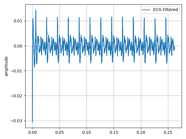
Figure 22. Other of my ECG signal acquired by the robot.

Figure 22. Signal spectrum analysis.

Once the capture and the pre-processing of the signal is done by applying stop-band filters, to remove the noise at 50 Hz, the next step is to convert it into an image, so it is necessary to remove the axes of the plot.

The image obtained is used to validate the model from our computer. At this point we have not used Openvino or the Neural Stick.

With a normal ECG classification result, my heart function is considered normal which is confirmed by my last medical check-up. The next step is to convert the model obtained from the training to files that openvino can understand. This process requires some important steps, the first one is to install Openvino, for which we refer to the instructions given by Intel. The installation steps vary according to our operating system (In my case, my operating system is Windows 10).

Once the Openvino is installed, the next step is to create a ventilation environment:

We create the environment: python3 -m venv openvinoWe activate the environment: .openvinoScriptsactivate

Once installed, the next step is to find the files that Openvino has installed:

C:Program Files (x86)IntelSWToolsopenvinodeployment_toolsmodel_optimizerinstall_prerequisites

Being within an environment, it does not allow us to install as --user the necessary requirements, so we modify the files. The first one is install_prerequisites we look for the word --user and we remove it. Once we have edited this file we can install the prerequisites.

With the installation completed with our model in.h5format, the next thing is to convert this model into a.pb model. To do this, we use the following code:

import tensorflow as tf from tensorflow.python.keras.models import load_model # Tensorflow 2.x from tensorflow.python.framework.convert_to_constants import convert_variables_to_constants_v2model = load_model("../KerasCode/Models/keras_model.h5") # Convert Keras model to ConcreteFunction full_model = tf.function(lambda x: model(x))full_model = full_model.get_concrete_function(  tf.TensorSpec(model.inputs[0].shape, model.inputs[0].dtype)) # Get frozen ConcreteFunction frozen_func = convert_variables_to_constants_v2(full_model)frozen_func.graph.as_graph_def() # Print out model inputs and outputs print("Frozen model inputs: ", frozen_func.inputs) print("Frozen model outputs: ", frozen_func.outputs) # Save frozen graph to disk tf.io.write_graph(graph_or_graph_def=frozen_func.graph,  logdir="./frozen_models",  name="keras_model.pb",   as_text=False)

This will return a file "XXXX.pb". Then, the next step is to look for this script mo_tf.py in the folder where Openvino was installed. Once in this folder, it is important to create a folder (if you want) that is called models and from the command terminal (cmd), we write this:

python mo_tf.py --input_model modelkeras_model.pb --input_shape [1,224,224,3] --output_dir model

If all goes well, we'll have to have these files at the end of this process:

• keras_model.bin
• keras_model.mapping
• keras_model (XML)
• labels.txt

With the acquisition system, the validation of the model with the captured ECG signal and the transformation of the.h5 model to Openvino compatible files, the following is to integrate this system into the company robot, as shown in figures 21, 22 and 23.

Figure 21. Components of the companion robot.

Figure 22. Front view of the companion robot.

Figure 23, Compain robot and NCS2

The company robot is built with a Raspberry Pi 4, as a control and process unit. It has two micro servos which control the ears and a servo for neck movement. In order to improve the expressiveness of the robot, it has been added a 24x8 LED Dot Matrix Module - Emo from the company sunfounder. A 3D model can be seen in Figure 24.

Figure 24. 3D model of the companion robot.

The robot control process is done using SPADE, which is a multiagent system platform written in Python and based on instant messaging (XMPP). This platform allows me to see my robot as an agent, that is to say, an autonomous and intelligent entity which is capable of perceiving the environment and communicate with other entities.

SPADE needs an XMPP server, so we decided to use Prosody's server that was installed on a pi raspberry. At the same time and in order to receive the messages that the robot sends when it finishes the signal analysis, I connected my smartphone to the XMPP server using the AstraChat application. This way the robot can send as messages the results of the analysis.

This communication is done through the passage of messages, similar to having a chat between different entities and allowing the user to be included in it.

State 1 is the initial state. State 2 is in charge of receiving messages from other agents or messages sent by the user using an XMPP client. State 3 is in charge of sending messages to other entities or to the user through the chat, and allows sending the result of the classification, that is, if the user has a heart problem. Finally, state 4 is in charge of controlling the robot.

The robot can be programmed to perform ECG signal capture. This capture can be done every two minutes, three, etc. It is important to note that the robot will capture the heart signal for one minute, during this period the robot does not perform any other action. In order that the user knows that the robot is in this state, the eyes of the robot are transformed into two hearts.

Once the capture process is completed, the robot sorts the captured signal and returns to the previous state. The result of the analysis is sent to the doctor or care center through the chat. The result of this validation can be seen below: